Understanding Synaptic Plasticity Algorithms

When synaptic plasticity algorithms were introduced to me, they were described alongside the leaky-integrate-and-fire model of neurons. I was confused at first because I conflated neuron models and the plasticity algorithms themselves. So right off the bat, these things should be distinguished. The leaky integrate-and-fire model is a computationally simple model of neuronal dynamics. Synaptic plasticity algorithms like spike-timing-dependent plasticity, the Oja learning rule, and the BCM rule are completely independent and they tell us how synaptic strengths change. So here, the focus is on the synapse. Or for the machine learning engineer, the weights. How does the brain learn if backprop isn't an option?

Spike-Timing-Dependent Plasticity

Spike-Timing-Dependent Plasticity, or STDP, takes the basic concept of Hebbian learning and parameterizes it. You might have heard the phrase "neurons that fire together, wire together." While this is often attributed to Donald Hebb, it's actually a later formalization of his ideas. In his influential 1949 book "The Organization of Behavior", Hebb proposed that when one neuron repeatedly participates in firing another, the connection between them strengthens. This was revolutionary at the time, but it left open a crucial question: what exactly counts as "repeatedly participates"? How close in time do the spikes need to be?

The discovery of STDP in the late 1990s, particularly through the groundbreaking work of Bi and Poo, provided a precise answer. Using cultured hippocampal neurons, they showed that the exact timing between pre-synaptic and post-synaptic spikes determines whether the synapse strengthens or weakens. The precision was remarkable - differences of just a few milliseconds could change the outcome.

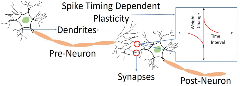
Here's how it works: when a pre-synaptic neuron fires slightly before a post-synaptic neuron (within about 20 milliseconds), the synapse between them strengthens. This makes intuitive sense - if neuron A consistently fires right before neuron B, then A might be helping to cause B's firing, so we should strengthen that potentially causal connection. On the flip hand, if the post-synaptic neuron fires before the pre-synaptic one, the synapse weakens. This also makes sense - if B is firing before A, then A probably isn't causing B's activity, so that connection might not be useful.

The graph above shows this relationship. Long term potentiation (LTP), or strengthening of the synapse, occurs in the right side where Δt (the time difference) is positive - meaning the pre-synaptic neuron fired first. Long term depression (LTD), or weakening, occurs on the left side where Δt is negative. The closer the spikes are in time, the stronger the effect.

This timing relationship can be described mathematically. For a positive Δt (pre-before-post): $\Delta w = A_+ \exp(-\Delta t/\tau_+)$

And for a negative Δt (post-before-pre): $\Delta w = -A_- \exp(\Delta t/\tau_-)$

The parameters in these equations control the shape of the learning window:

• $A_+$: Maximum amount of strengthening (potentiation)
• $A_-$: Maximum amount of weakening (depression)
• $\tau_+$: How quickly the strengthening effect falls off with time
• $\tau_-$: How quickly the weakening effect falls off with time

You can explore how these parameters shape the learning rule using the interactive visualization below. Try adjusting the time constants and amplitudes to see how they affect the timing window:

Biological Significance and Computational Properties

What makes STDP particularly fascinating is how it combines biological plausibility with computational elegance. Unlike backpropagation in artificial neural networks, STDP is local - each synapse only needs information about the timing of its pre- and post-synaptic neurons' spikes. There's no need for some external system to compute gradients and propagate them backward through the network. This locality makes it a much more plausible mechanism for how real brains might learn.

The discovery of STDP has been validated across many brain regions and species, from the hippocampus (crucial for memory formation) to sensory systems. The exact shape of the learning window can vary - some synapses show stronger depression than potentiation, others the reverse. This variability might reflect different computational needs in different brain areas.

STDP also provides a mechanism for learning temporal sequences and detecting causality in neural circuits. If activity consistently flows through a particular sequence of neurons (A→B→C), STDP will naturally strengthen those connections in that specific order. This property makes it particularly relevant for tasks like learning motor sequences or processing temporally structured sensory inputs.

The implications go beyond biology. STDP has inspired new approaches in neuromorphic computing - computer architectures that try to mimic the brain's efficiency. Traditional deep learning typically updates weights in discrete steps using globally computed gradients. STDP suggests a different approach: continuous local updates based on spike timing. This could lead to more efficient, more biological learning systems.

However, it's important to note that STDP isn't the whole story of synaptic plasticity. The brain uses multiple mechanisms operating at different timescales and responding to different cues. STDP is just one piece of the puzzle - albeit a fascinating one that bridges the gap between the millisecond-scale timing of neural spikes and the emergence of learned behavior.